478 stores · 85 suppliers · 1,265 SKUs · 3.27M predictions

Retail AI that
catches what
humans can't see.

HyperShelf DemandSense v2 is a full-stack retail intelligence pipeline LightGBM probabilistic demand forecasting, Random Forest phantom inventory detection, and a locally-served LLM that explains real supply chain decisions without hallucinating a single number. Engineered by an AI & Machine Learning Engineer and MS student at the University at Buffalo.

$47.4M
Revenue risk tracked
24.06%
WAPE — vs ~32% baseline
14,041
Phantom SKUs flagged
188,143
Stockout events prevented
89.75%
P90 demand coverage
CRITICAL 6,544 SKUs need immediate order REVENUE AT RISK $47.4M network-wide WAPE 24.06% vs ~32% moving average baseline P90 COVERAGE 89.75% — target 88–92% PHANTOM INVENTORY 14,041 candidates across 478 stores BLACK FRIDAY BIAS -1.72 — model predicted 17 for every 10 sold REVENUE RECOVERED $275.6M vs old static reorder policy SAFETY STOCK Dynamic SS = Z × √(LT·σD² + D²·σLT²) × SF CRITICAL 6,544 SKUs need immediate order REVENUE AT RISK $47.4M network-wide WAPE 24.06% vs ~32% moving average baseline P90 COVERAGE 89.75% — target 88–92% PHANTOM INVENTORY 14,041 candidates across 478 stores BLACK FRIDAY BIAS -1.72 — model predicted 17 for every 10 sold REVENUE RECOVERED $275.6M vs old static reorder policy SAFETY STOCK Dynamic SS = Z × √(LT·σD² + D²·σLT²) × SF
The problem

A retail network flying
completely blind.

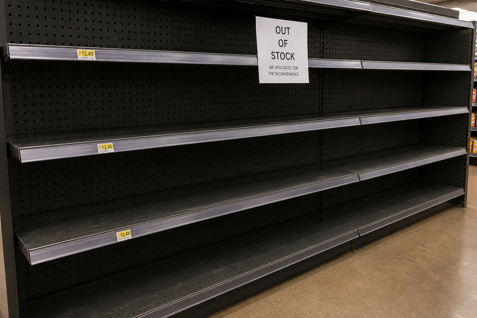
It’s a Friday evening. A family walks into a store to buy their favorite brand of premium juice for the weekend. The shelf is completely empty. They leave and buy it at a competitor's store.

The store manager investigates and finds the system says 0 stock. They place an emergency order immediately, but the upstream supplier has an 11-day lead time. The next weekend arrives foot traffic is up 40% for Saturday shopping, but the product still hasn't arrived. The shelves remain empty. The cycle repeats.

Meanwhile, across 478 stores, $47.4M in revenue is silently disappearing. Not from theft. Not from damage. From a forecasting model that treats every day the same as a 30-day moving average that has no concept of weekends, promotions, lead time variability, or demand uncertainty. When Black Friday hits and stores clear shelves in 4 hours, the model keeps predicting the same volumes it saw last month. For every 10 units sold, it predicted 17. Bias: -1.72.

The safety stock policy was Target = μ. Average demand, nothing more. No buffer for uncertainty. No tier-based service level. No model for what happens when a supplier delivers 3 days late into a peak week. The result: stockouts that were entirely predictable if you had the right model.

The core problem: Legacy systems produce numbers, not intelligence. They tell you what demand was. They don't tell you what it will be, how uncertain that prediction is, where ghost inventory is locking up capital, or what to do about any of it. HyperShelf DemandSense v2 was built to fix all four.
Empty Store Shelf
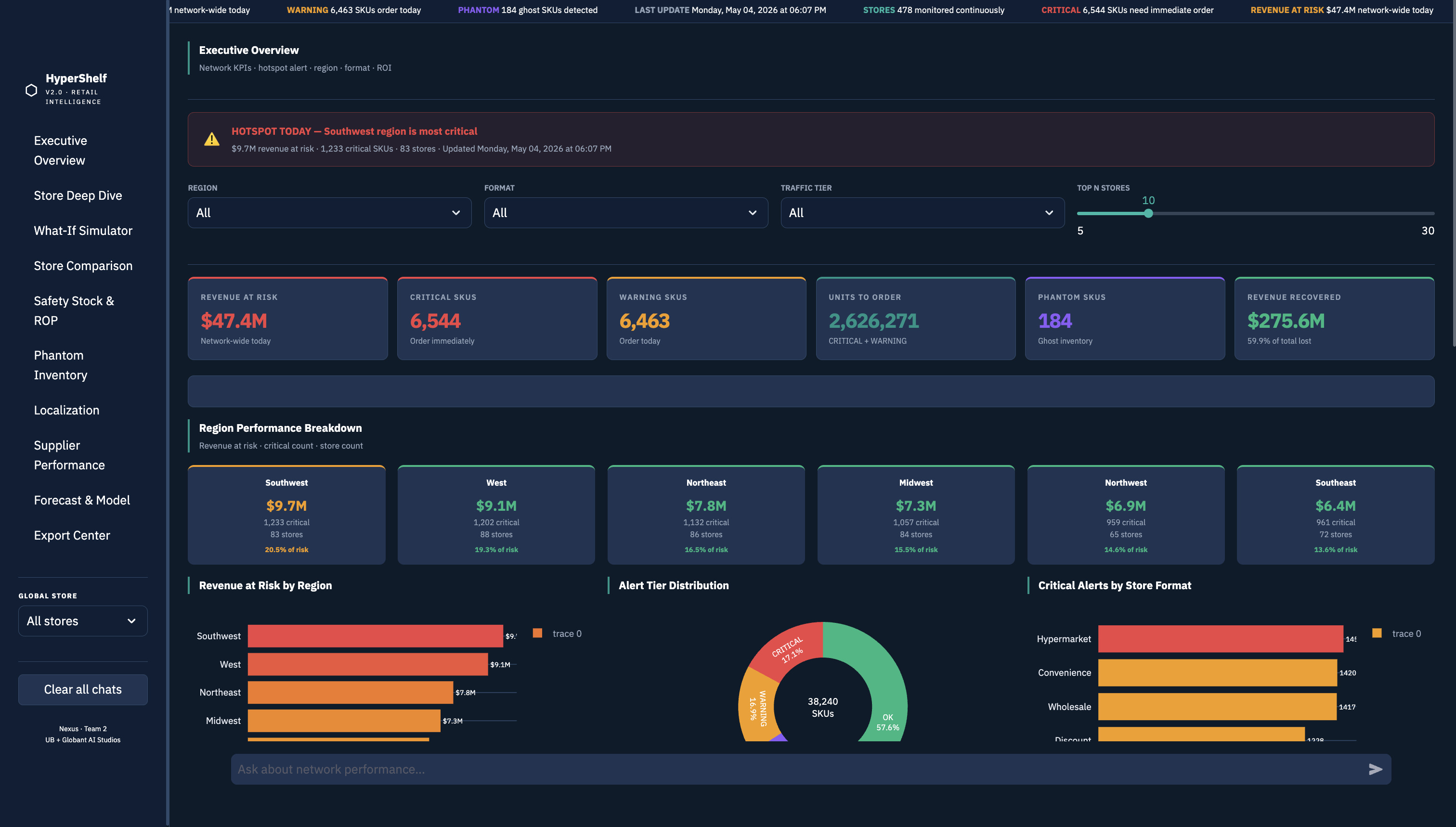
Dashboard Critical Alerts
32.7%
P90 demand coverage under the legacy model. Against a 90% target. The system was calibrated for a world where demand is perfectly predictable.
97.8u
Average shortage per SKU during promotional events. The old model had no promo depth or demand lift features — it was blind to every sale you ran.
$85.6M
Revenue leakage identified at baseline. The system wasn't losing money through waste it was losing through demand it didn't know existed.
0
Safety stock units in the old policy. Reorder point = μ. No uncertainty buffer. No tier-based service level. No protection against supplier delay.
Demand Forecasting

LightGBM why gradient
boosting wins in retail.

Retail demand is non-linear, non-stationary, and event-driven. A 30-day moving average assumes yesterday predicts tomorrow. LightGBM assumes nothing it learns from the interaction between day-of-week, promotional depth, lag velocity, and store format simultaneously, capturing patterns that no linear model can represent.

System Architecture Diagram

Why LightGBM specifically

Gradient boosting builds an ensemble of trees sequentially each tree corrects the residual errors of the previous one. For retail, this matters because demand drivers interact in complex, non-additive ways: a Saturday promotion in a Premium store during summer hits differently than the same promotion on a Tuesday in a Medium store in winter. Decision trees capture those interactions natively through splits. Linear models require you to specify them manually, and you'll miss most of them.

LightGBM specifically rather than XGBoost was chosen for its leaf-wise tree growth on 4.58 GB of training data. Leaf-wise growth reduces error faster per tree than level-wise, which matters when training on 18.3 million time-series observations where every additional epoch is computationally expensive.

Probabilistic output: Instead of predicting a single demand number (P50), the model uses quantile regression to output P10 (low demand scenario), P50 (median expected), and P90 (high demand scenario). The P90 drives safety stock decisions order at the upper bound to protect against demand spikes. This alone restored P90 coverage from 32.7% to 89.75%.

22 features what each does

Segment featurescategory, foot_traffic_tier, region, store_format, price_band — the model learns separate demand baselines per segment. Premium stores in the Southwest have fundamentally different demand curves than Low-tier stores in the Northeast.
Temporal featuresdow, month, weekofyear, is_weekend — retail demand is weekly-seasonal. Saturday demand for beverages is 40% higher than Monday. Without weekday features, the model can't capture this and over-orders on Mondays, under-orders on weekends.
Lag featureslag_1, lag_7, lag_14, lag_28 — give the model memory. lag_7 says "what did this SKU sell exactly one week ago?" This captures the weekly demand cycle. roll_mean_7/28 smooth out noise. roll_std_7 captures demand volatility — high std → wider safety stock band needed.
Promo features (V2.2)discount_pct, demand_lift_factor, promo_depth_x_flag, promo_lift_x_flag — the legacy model had zero promo awareness. A 40%-off event causing 3× demand looked identical to a regular Tuesday. These 4 features reduced promotional shortages from 97.8 units average to near zero
Stockout proxy (V2.2)lost_units_proxy, stockout_flag — when a shelf is empty, sales are zero even if demand is high. Without this, the model trains on censored observations and under-forecasts during restocking. The proxy estimates true demand during stockout periods.

The fundamental error how money is lost

In supply chain forecasting, the basic calculation defines exactly how you lose money:

Forecast Error Definition
Error = Actual Demand - Forecast
Positive Error (Under-forecasting): Actual > Forecast. Leads directly to stockouts and lost sales.
Negative Error (Over-forecasting): Forecast > Actual. Leads to excess inventory, locked capital, and waste.

Our analysis revealed that the old moving average model heavily skewed toward positive errors during high-footfall promotional events. This under-forecasting is what drove the massive $85.6M in baseline revenue leakage.

The true demand problem the evolution of the WAPE metric

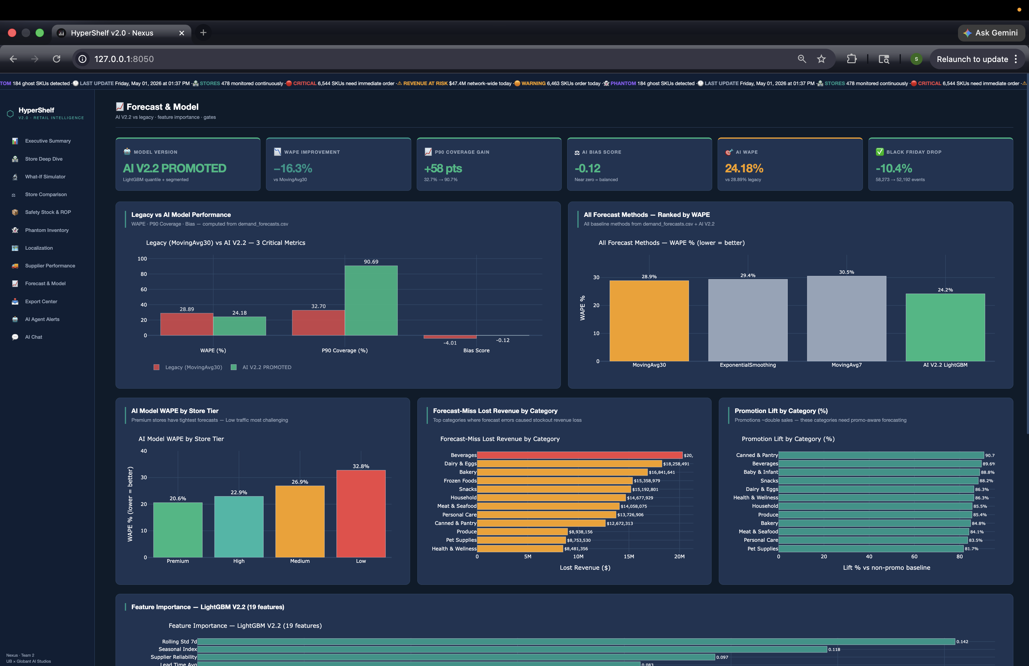
The legacy moving average model had a massive error rate of around 32%. We initially built a LightGBM model that brought the standard WAPE down to 24.18%. However, we realized this was a false success. The standard WAPE calculation uses observed sales as the target. But when shelves are empty, sales are zero regardless of actual demand. This censors the training signal. When we corrected the target to True Demand (actual sales + lost units), we found that the 24.18% model actually had an error of 28.19%. We then retrained the pipeline completely on the True Demand target, successfully bringing this much harder metric down to a final 24.06%.

1. Legacy Moving Avg

~32.00% The old baseline. Completely blind to promotional volatility and lead time variation.

2. LightGBM V1 (Biased)

24.18% Our first model. Looked like a huge win, but it was trained on observed sales, masking stockouts.

3. The Reality Check

28.19% When we corrected the target to True Demand (sales + lost units), the error of V1 jumped to 28.19%.

4. Final LightGBM V2

24.06% Retrained on the corrected True Demand target, finally bringing the true error down to 24.06%.

Tiered service levels because not all SKUs are equal

Store tierTarget CSLZ-scoreFormulaWhy this tier
Premium97.5%1.960μ + 1.96σ√LHigh-value products, high-footfall stores. A stockout here loses $2,000+/day per SKU.
High97.5%1.960μ + 1.96σ√LHigh foot traffic. Revenue at risk per stockout justifies higher carrying cost buffer.
Medium95.0%1.645μ + 1.645σ√LBalanced cost vs service level. 95% means stockout 1 in 20 replenishment cycles.
Low95.0%1.645μ + 1.645σ√LLower volume, cost-sensitive. Carrying excess safety stock here destroys margin.

The NULL promotion bug why only 1,434 rows had promo data

promotions.csv stored all-store promotions with store_id = NULL. A direct join on store_id dropped every all-store promo from the training data — leaving only 1,434 non-zero discount_pct rows out of 24 million. The model trained as if almost nothing was ever on promotion. Fix: detect NULL store_id rows, expand them to every store in the network before joining, then re-merge with store-specific promos. The promo feature went from near-useless to one of the top-5 by feature importance.

Before fix: 1,434 rows with non-zero discount_pct out of 24M rows (0.006%)
After fix: millions of rows with accurate promo depth — top-5 feature by importance
Impact: promotional shortage reduced from 97.8 units average to model-aware replenishment
Phantom Inventory Detection

Random Forest hunting
ghosts in the data.

Phantom inventory is product the system believes exists but physically doesn't — miscounted, mislabelled, lost behind shelves. The system places no reorders because inventory shows available. The customer finds empty shelves. 14,041 such SKUs were flagged across 478 stores with High/Medium/Low confidence.

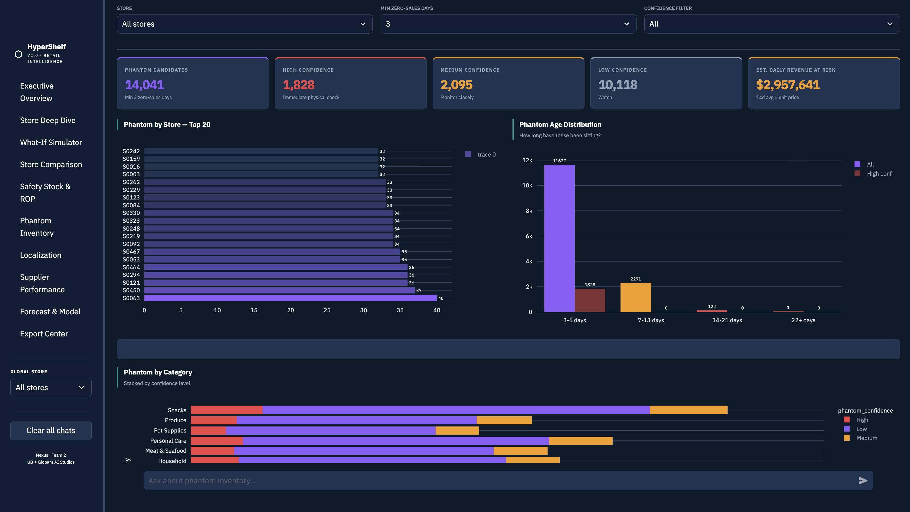
Phantom Inventory Aisle Check List

Why Random Forest for this problem

Phantom detection is a binary classification problem with highly non-linear decision boundaries. A product that sold 50 units last week and zero this week is probably not a phantom — maybe it's a slow week. But a product that shows 200 units available, matches 3 phantom detection rules, and has had zero sales for 14 consecutive days is almost certainly a ghost. Random Forest captures these compound patterns through feature interactions across many trees, naturally handling class imbalance and providing confidence scores through vote proportion rather than a hard threshold.

Why F2, not F1 or accuracy: In phantom detection, a False Negative means missing a real ghost — that product stays "in stock," no reorder fires, shelves stay empty, revenue is lost. A False Positive means sending an associate to check an aisle that turns out to be fine — 2 minutes wasted. The cost asymmetry is extreme. F2 weights recall twice as heavily as precision, accepting more false positives to catch more real phantoms.

4 engineering decisions that made it work

Label sourceOriginal labels came from the stockout table, which only captures complete stockouts — shelves fully empty. Ghost inventory is different: the system shows stock, but nothing sells. Labels were rebuilt from inventory-sales mismatch: stock present in system + zero observed sales velocity. This fundamentally changed what the model was learning.
All 3 phantom rulesThree detection rules existed as separate logic checks. All three were included as explicit model features: consecutive zero-sales day count, inventory-to-forecast ratio, and velocity drop score. The RF learns which rules matter per product type not all phantoms fail all three rules simultaneously.
F2 PR-curve thresholdThe default threshold of 0.55 maximised precision (flagging fewer, more certain phantoms). But precision is the wrong objective here. F2 threshold from the Precision-Recall curve was optimised for recall × 2. This catches more real phantoms at the cost of more aisle checks the right trade.
Lag featureslag_1, lag_7, lag_14 added as features. A product with zero sales today may have sold well last week — it's not a phantom, just slow. A product with zero sales across all three lag windows, with inventory showing available, is almost certainly a ghost. Temporal context makes the difference.
Supply chain integration

Why the old formula
was wrong and what replaced it

Probabilistic forecasts are only valuable if they drive decisions. LightGBM's μ and σ outputs feed directly into a stochastic replenishment policy that replaced the naive old system. The change is not cosmetic — it fundamentally alters how inventory buffers are calculated.

The old policy what was wrong

The legacy reorder policy was:

Old policy (static)
Target = μ × Lead Time

This assumes two things that are both wrong in retail: (1) demand is perfectly predictable — that σD = 0, that tomorrow will look exactly like the 30-day average. And (2) suppliers are perfectly reliable — that σLT = 0, that a supplier who promised 7 days will always deliver in exactly 7 days. The formula buffers for neither. When a supplier delivers 3 days late into a Black Friday week where demand is running 40% above forecast — which is exactly when it will happen the policy has no protection. Stockout is mathematically guaranteed.

The result: 0 safety stock units in the old policy. P90 coverage of 32.7%. $85.6M in leakage.

The new formula what it accounts for

New policy (stochastic)
SS = Z × √(LT × σD² + D² × σLT²) × SF
Target = μ × LT + SS
Z — service level factor, tier-based (1.645 for Medium/Low, 1.960 for Premium/High)
LT — average supplier lead time in days (from supplier scorecard)
σD — daily demand standard deviation — from LightGBM's distribution output
D — average daily demand μ — from LightGBM P50 forecast
σLT — lead time standard deviation from supplier delivery history
SF — seasonal factor — from model's demand_lift_factor feature

The formula has two variance terms inside the square root. LT × σD² captures demand uncertainty during the lead time period. D² × σLT² captures lead time uncertainty — what happens when a supplier is late. Both terms matter. A highly reliable supplier serving volatile demand needs more safety stock than an unreliable supplier in a predictable category. The old formula captured neither. The new formula captures both, scaled by the tier's service level Z-score.

Black Friday backtest result: With dynamic safety stock applied and the Champion model promoted, the policy backtest over Black Friday and Christmas showed an 8.33% reduction in stockout events and a 4.41% reduction in lost units compared to the old policy running over the same period. The formula isn't theoretical — it was validated against the hardest weeks in the retail calendar.
LLM Architecture & Dashboard

AI embedded in
every single page.

Rather than just a static reporting dashboard, HyperShelf v2.0 features ubiquitous Agentic AI We built two distinct layers: a global Standalone AI Chat for network-wide questions, and localized AI Explainers embedded directly into all 10 dashboard pages (Forecast, Stockouts, What-If, etc.).

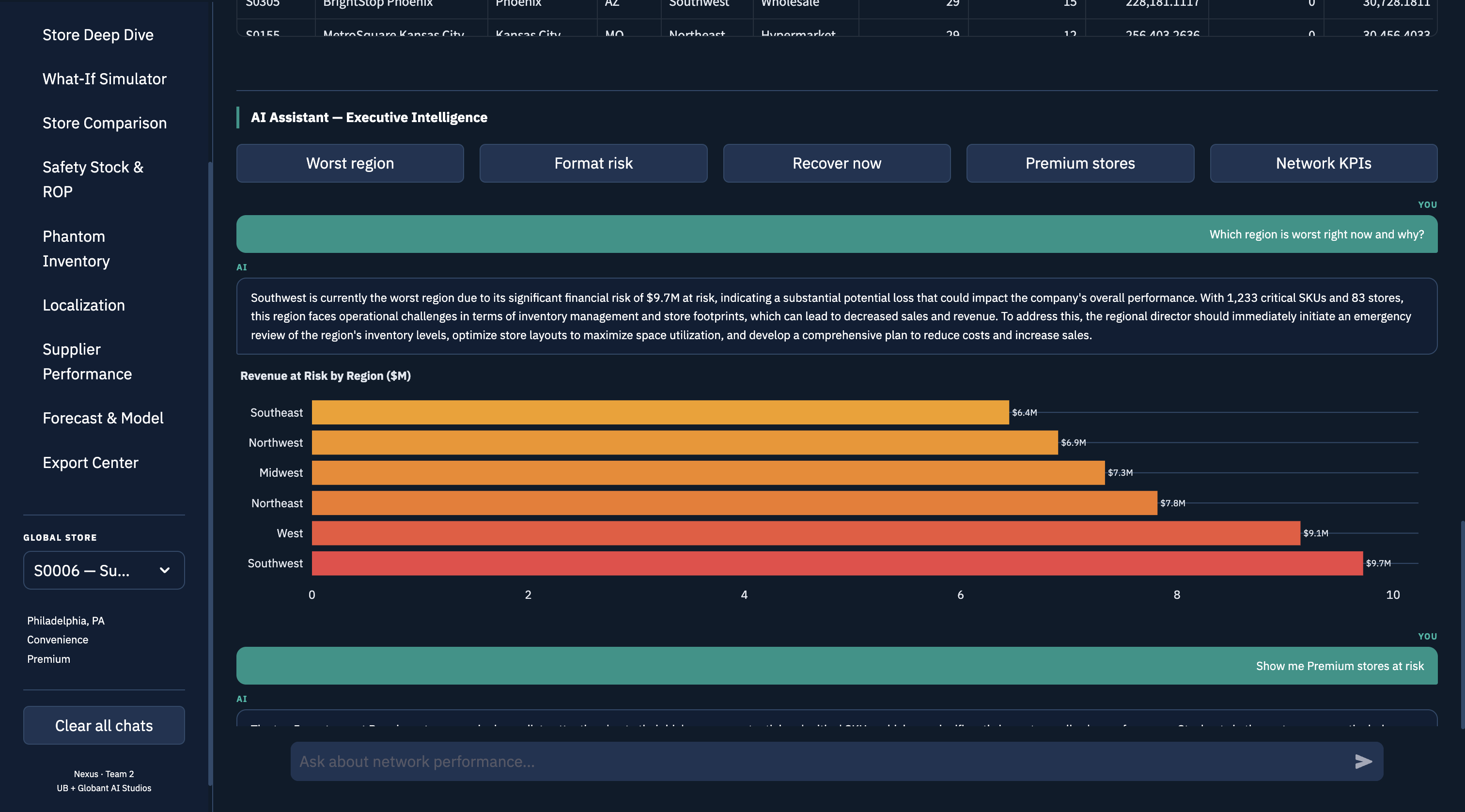
Standalone Conversational AI Chat

Interactive Dashboard AI Modules

The full question-to-answer flow

01
User question
"Why did WAPE spike on Black Friday?"
→
02
Python router
600-line answer() — keyword + regex intent detection routes to correct path
→
03
Data fetch
Python queries database and computes exact math natively
→
04
Facts text
Structured summary passed to LLaMA — exact numbers only — no raw data
→
05
LLaMA 3.2
Explains retail demand forecasting context — adds reasoning — temperature 0.2
→
06
User answer
"Black Friday: WAPE 32.3%, Bias -1.72. For every 10 units sold, model predicted 17..."

Why LLaMA 3.2 3B — and what it's actually for

LLaMA 3.2 3B is a 3-billion parameter language model served locally via Ollama with sub-2 second response time and zero API dependencies. It wasn't chosen for its ability to remember retail data — it was chosen for its ability to explain patterns that Python computes.

Python is better at: exact arithmetic, sorting, filtering, reading files, computing means and percentages. LLaMA is better at: explaining why Health & Wellness is harder to forecast than Meat & Seafood in conversational language, connecting "Bias -1.82" to "Post-Christmas demand collapse," adding retail domain context that would require 50 lines of hardcoded explanations if done in Python.

The hybrid architecture captures both strengths. Python computes "Health & Wellness: WAPE 23.4%, 90,343 training rows, Bias -0.10." LLaMA receives those exact numbers and explains why seasonal health trends and promotional volatility make this category structurally harder to model.

What Python doesReads CSVs, computes exact values, sorts, filters, identifies spike weeks, builds structured text summary. Never wrong on numbers it reads them from the file.
What LLaMA doesReceives the structured text summary and explains the retail context. Adds domain reasoning: "why Black Friday breaks forecasting models" or "why ordering at P90 protects against demand uncertainty." Temperature 0.1 for facts, 0.2 for explanations.
What LLaMA cannot doSee the raw 3.27M row prediction file. Compute anything. Invent numbers not in its prompt. The system prompt explicitly says: "Answer ONLY using the data above. Do not calculate or estimate."
Why this works at scaleYou can't pass 400MB of CSV to a 3B model. Python compresses the relevant answer into a 200-word summary. LLaMA explains those 200 words. The 3B parameter constraint becomes irrelevant because the model is never asked to retrieve only to explain.

4 engineering challenges in the LLM layer

Challenge 01 — Routing hallucination
LLaMA answered forecast questions with replenishment tool output
The model answered "Which category forecasts worst?" by inventing WAPE numbers using order quantities, with store IDs like S9999 that don't exist in any CSV
Without strict routing, LLaMA reached for the nearest available tool replenishment data and built plausible-sounding answers from it. Fix: A 600-line answer() routing function with keyword + regex intent detection. The WAPE handler sits at line 241, before any replenishment handler can intercept. Forecast questions hit the forecasting path first, always. Routing is explicit, not emergent from the model's understanding.
Challenge 02 — Context injection at 3.27M rows
Raw retail data cannot fit in a 3B model's context window
Asking about store-level WAPE got generic responses — the model had no actual data to reason about and invented metrics that sounded plausible but were completely fabricated
The solution is never passing raw data to the LLM. Fix: Python reads every CSV, computes the complete answer, formats it as structured facts ("Health & Wellness: WAPE 23.4%, 90,343 rows, Bias -0.10"), and passes only that 200-word summary to LLaMA. The model receives a compressed structured brief, not 400MB of tabular data. It explains, not retrieves.
Challenge 03 — Intent ambiguity across question types
Ambiguous questions hit the wrong handler, producing confident wrong answers
"What should I order?" sometimes returned demand forecast data instead of replenishment quantities — partially correct data, answering a completely different question than asked
Retail questions share vocabulary across domains "order" appears in both forecast and replenishment contexts. Fix: Priority-ordered routing. The WAPE spike handler checks its keywords first. If it matches, the question never reaches any other handler. Each domain has a fixed keyword set and explicit precedence order the most specific handlers are checked before general fallbacks.
Challenge 04 — Temperature calibration
High temperature produced inventive, confident, completely wrong answers
At temperature 0.7, LLaMA invented store IDs (S9999), revenue figures ($184,200 — never in any CSV), and a supplier fill rate of 87.3% for a supplier that doesn't exist in the scorecard
LLaMA 3.2 3B at high temperature treats domain jargon as creative latitude. Fix: Temperature 0.1 for all answers that cite specific numbers WAPE values, stockout counts, supplier names, revenue figures. Temperature 0.2 for explanatory text where phrase variation is acceptable and harmless. The model adds retail expertise around Python-computed facts. It never computes the facts itself.
"Python finds the exact number.
LLaMA explains what it means.
The user just gets the answer."
CORE ARCHITECTURE PRINCIPLE · HYPERSHELF DEMANDSENSE V2
Dashboard — 10 pages with AI

Every page has
its own AI module

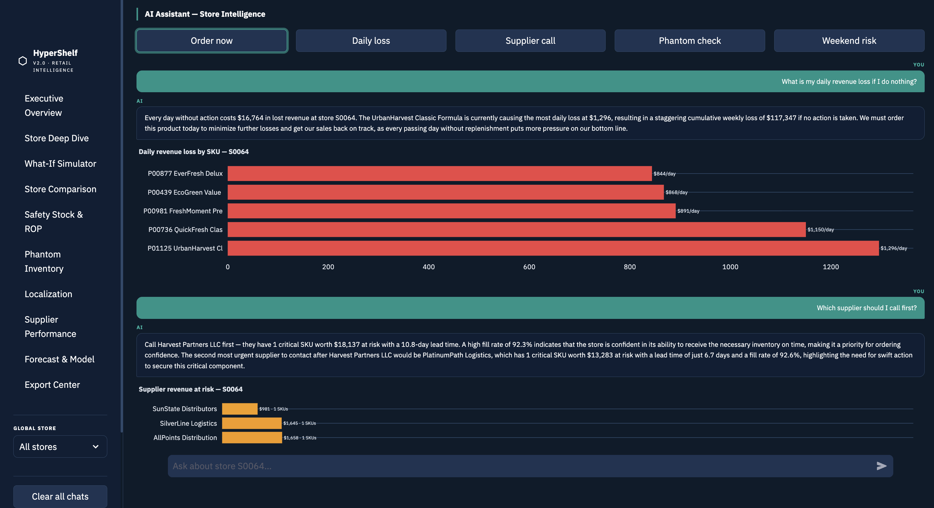
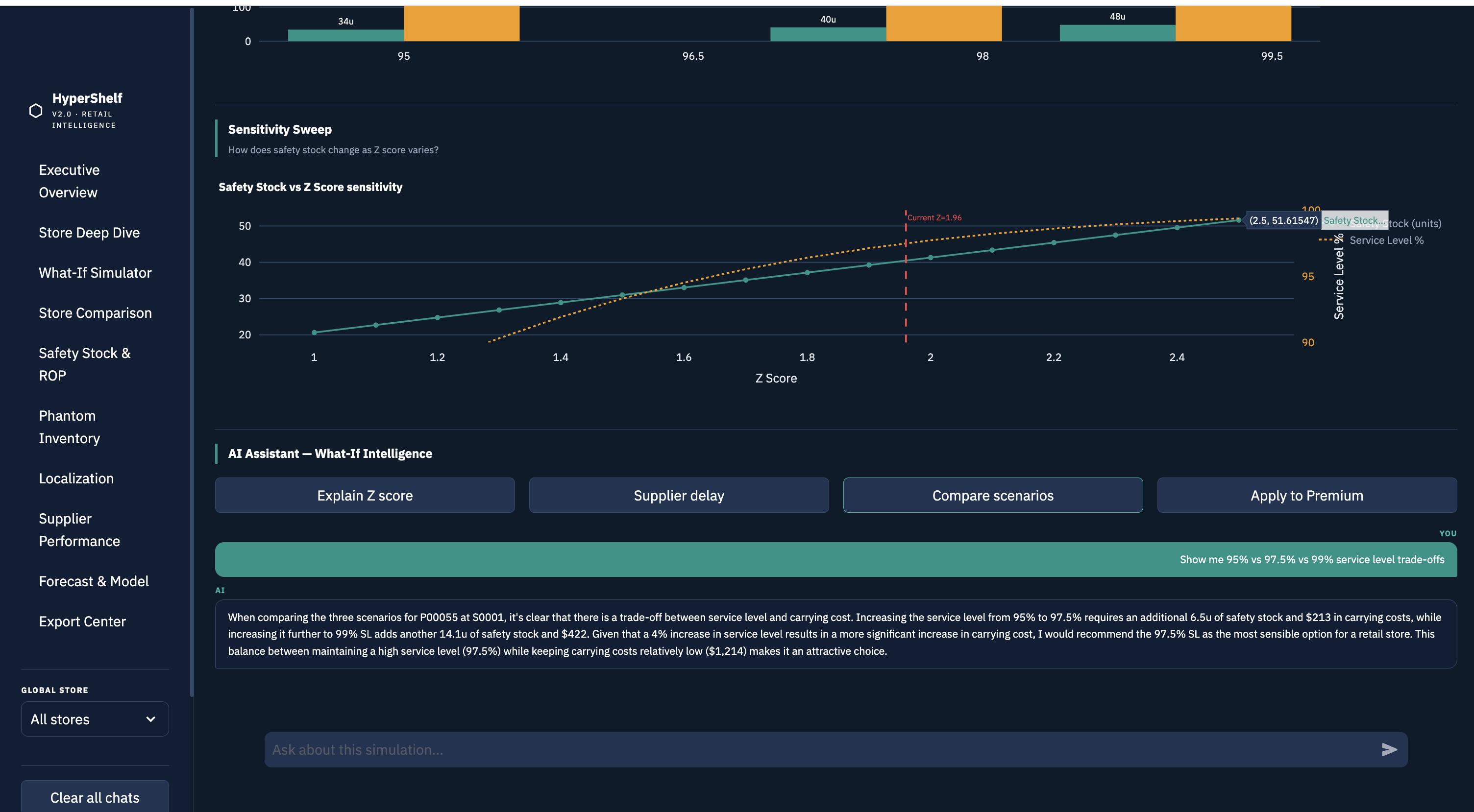
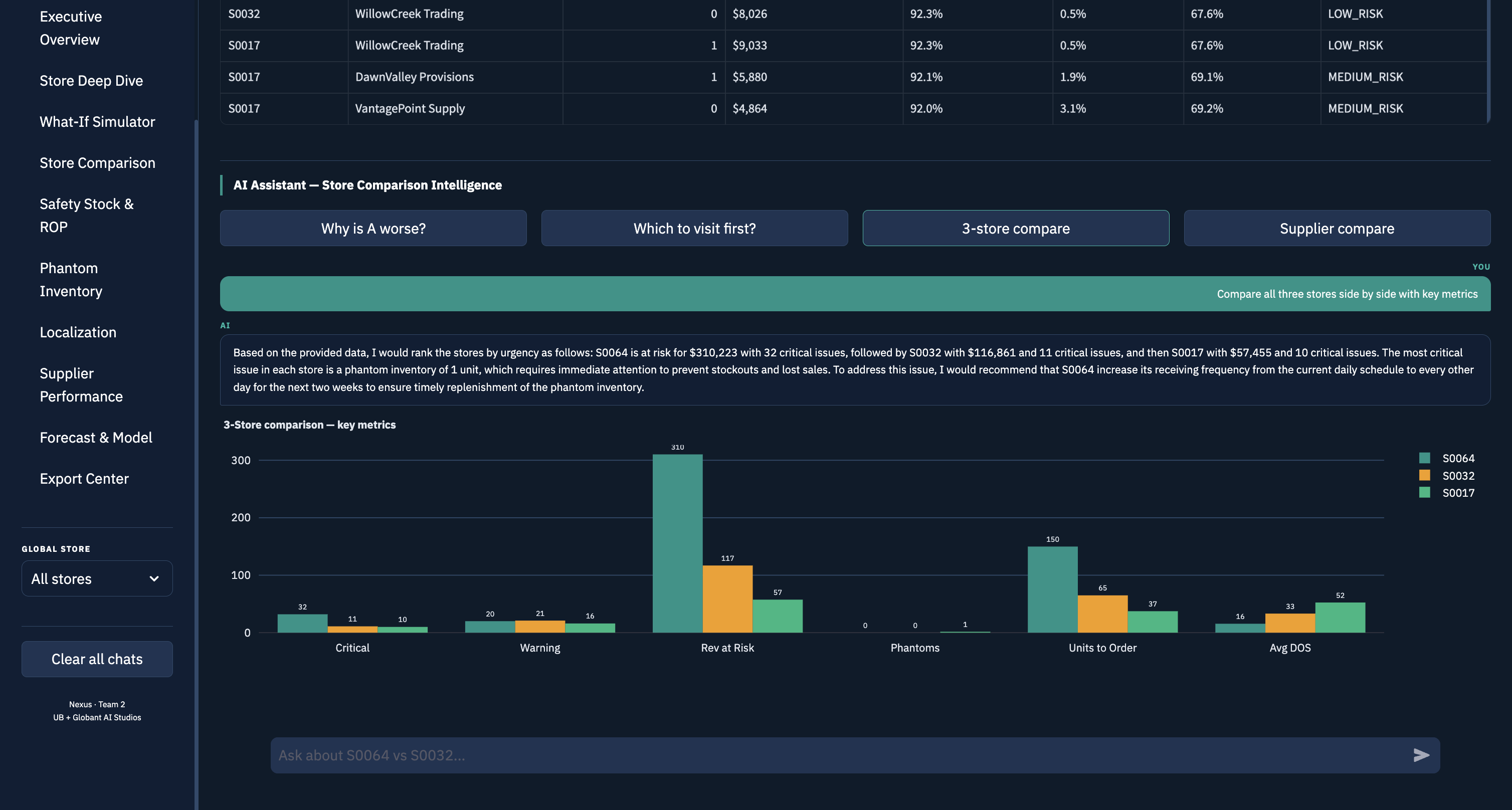
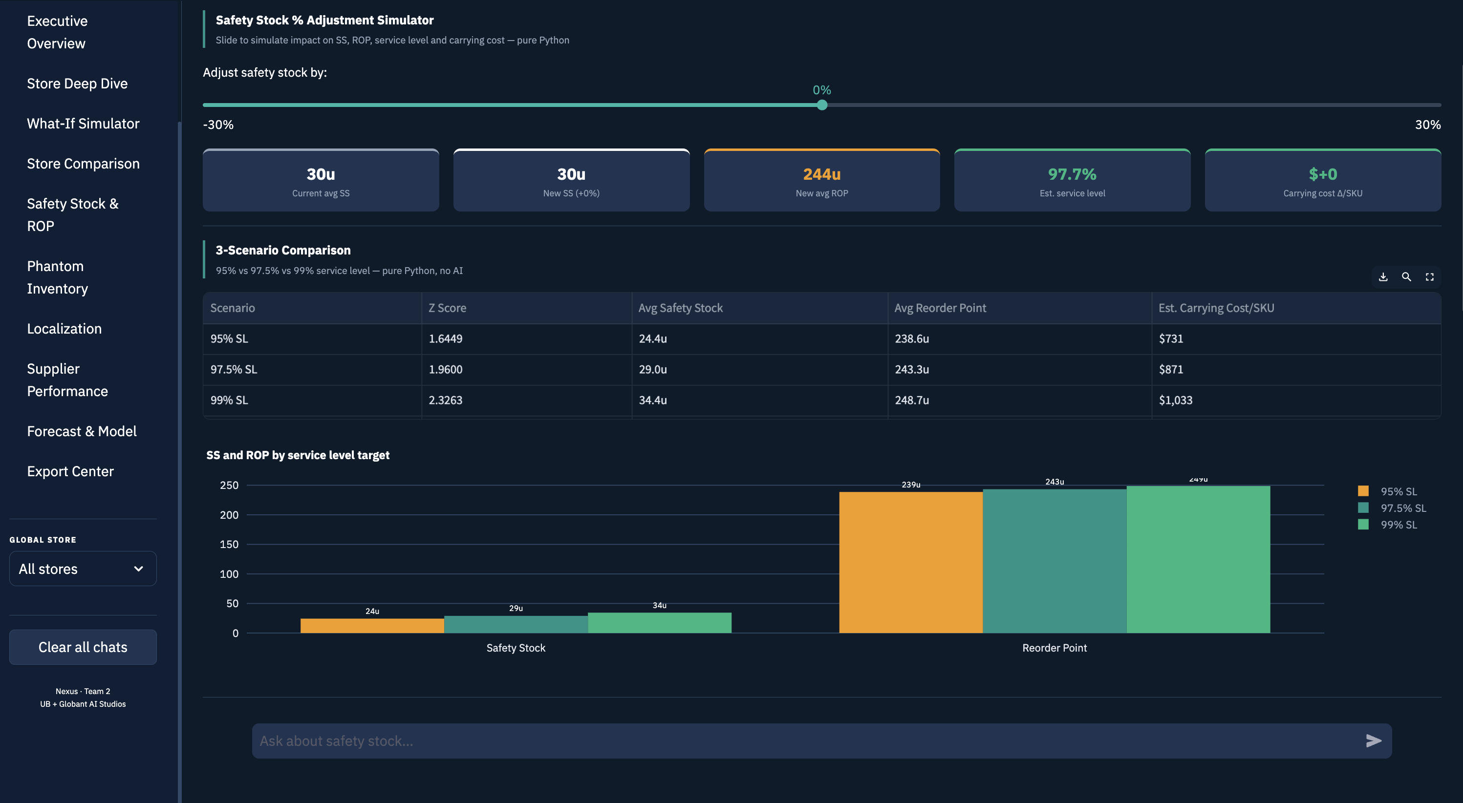
Each dashboard page runs its own Python AI module 10 separate files, each with intent routing, data fetching, and Plotly chart generation inline in the chat response. Quick reply buttons pre-wire the most useful questions. No page says "I don't know" every answer starts from real data.

Executive Overview
Executive Overview
Live network ticker. Region/format/tier filters. ROI simulator with Z-score slider. Top N urgent stores sorted by urgency score.
AI: "Southwest: $9.72M at risk · 2,341 CRITICAL · 83 stores. Superstore format drives 38% of total risk. Order 80% of critical SKUs today → $37.9M recoverable at 97.5% SL."
Store Deep Dive
Store Deep Dive
4 dropdowns. Days-of-supply gauges per CRITICAL SKU. Daily revenue loss if no order placed. Live alert table sorted by priority score (F1–F5 weighted).
AI: "$18,234/day lost if no action at S0064. Top loss: CoastalFarms Juice $4,102/day. Call VantagePoint Supply first — 16-day lead, stock arrives May 15."
What-If Simulator
What-If Simulator
6 sliders updating live. Safety stock, reorder point, service level, effective lead time, carrying cost all recalculate instantly. Sensitivity sweep chart.
AI: "At Z=1.96 (97.5% SL): SS 85u, ROP 295u, carrying cost $2,125/month. Going to 99% adds 16u more stock and $400/month — justified for Premium SKUs."
Store Comparison
Store Comparison
3-store selector. 5-factor priority breakdown (F1=tier, F2=revenue, F3=DOS, F4=supplier, F5=seasonal). Supplier 4-factor scorecard side by side.
AI: "S0064 worse: $310K vs $223K. Root cause: F4 supplier risk (InlandEmpire fill 91.6%, late 68%) and F3 DOS urgency running out 2.2× faster. Visit S0064 first."
Safety Stock & ROP
Safety Stock & ROP
SS% adjustment slider. Below-ROP product table with capital impact. Old vs AI policy comparison by store tier. 3-scenario SS comparison table.
AI: "Reducing SS by 10% saves $2.1M carrying cost but raises stockout probability from 2.5% to 5.8% for Premium stores. Not recommended for this tier."
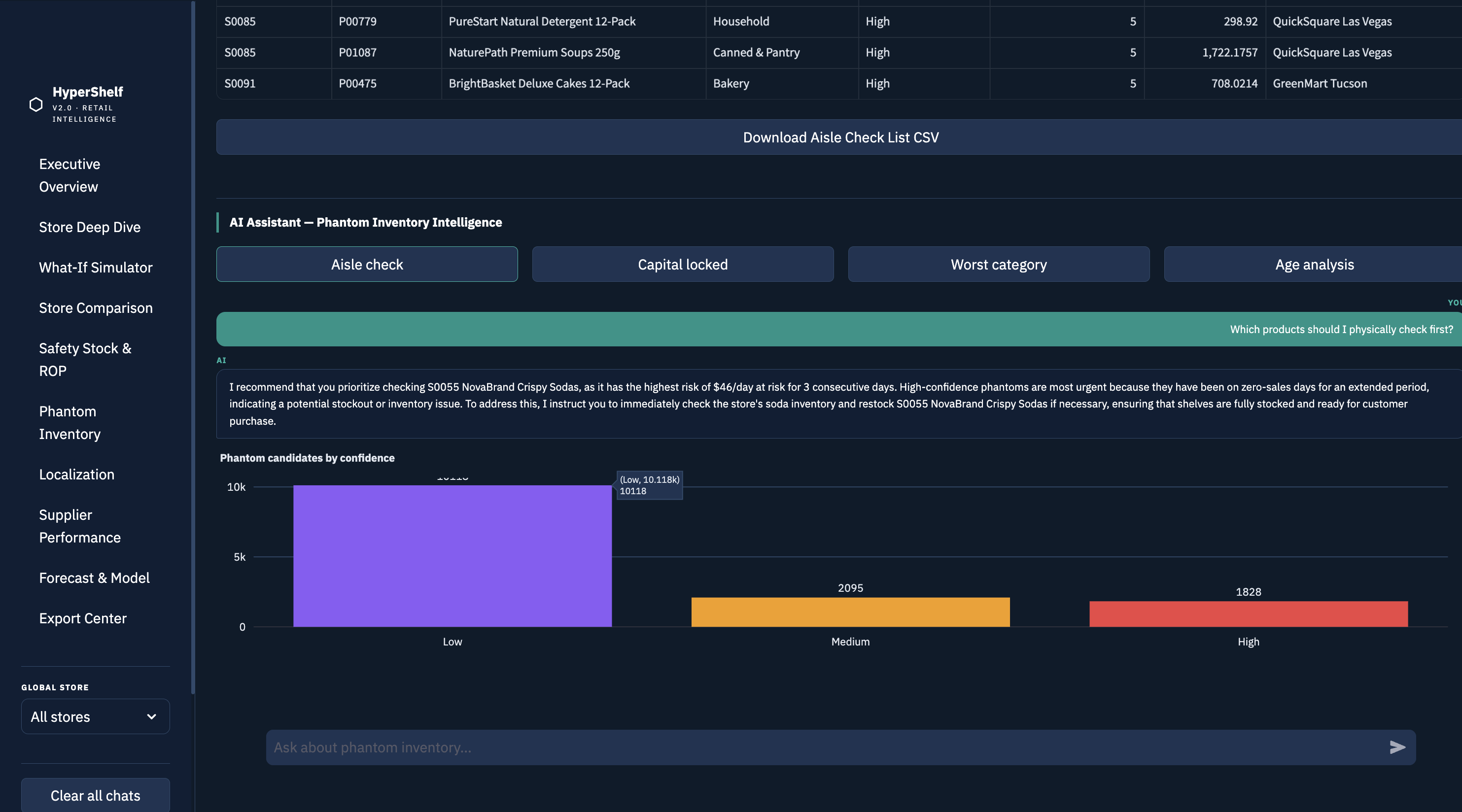
Phantom Inventory
Phantom Inventory
3 dropdowns. Age distribution by consecutive zero-sales days. Aisle check list. High/Medium/Low confidence breakdown by category. CSV download for store teams.
AI: "PrimePick Light Wipes 1kg — 14 zero-sales days, $11,573 capital locked, High confidence. Send associate to Check planogram immediately. 8 SKUs need physical verification."
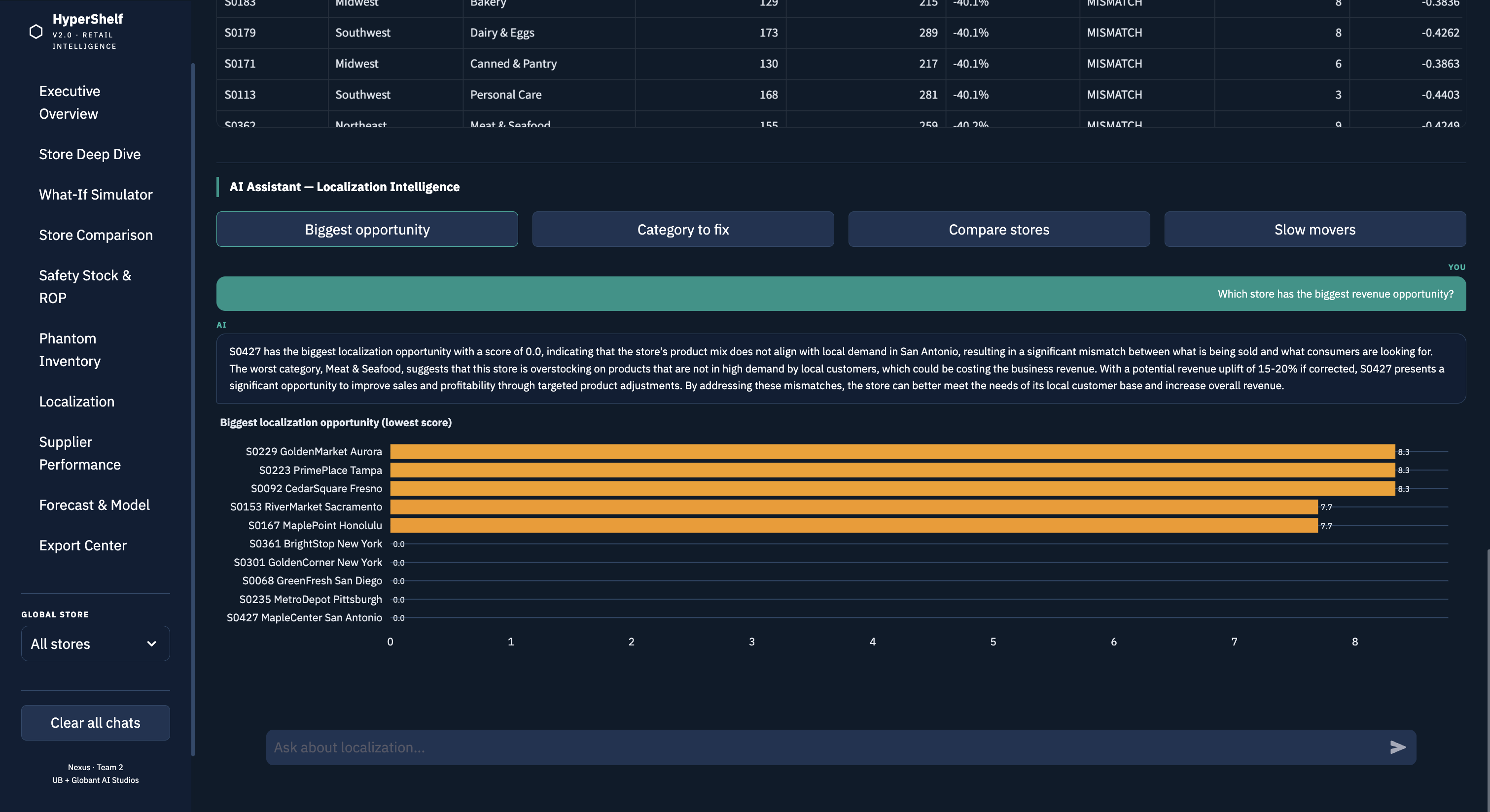
Localization
Localization
Store A vs Store B revenue mismatch. Category performance vs region average. Slow-mover capital efficiency. Revenue uplift potential by store.
AI: "S0064 has the biggest opportunity: Meat & Seafood 10 mismatched categories vs region average. Estimated uplift $500K–$750K/year if product mix is corrected."
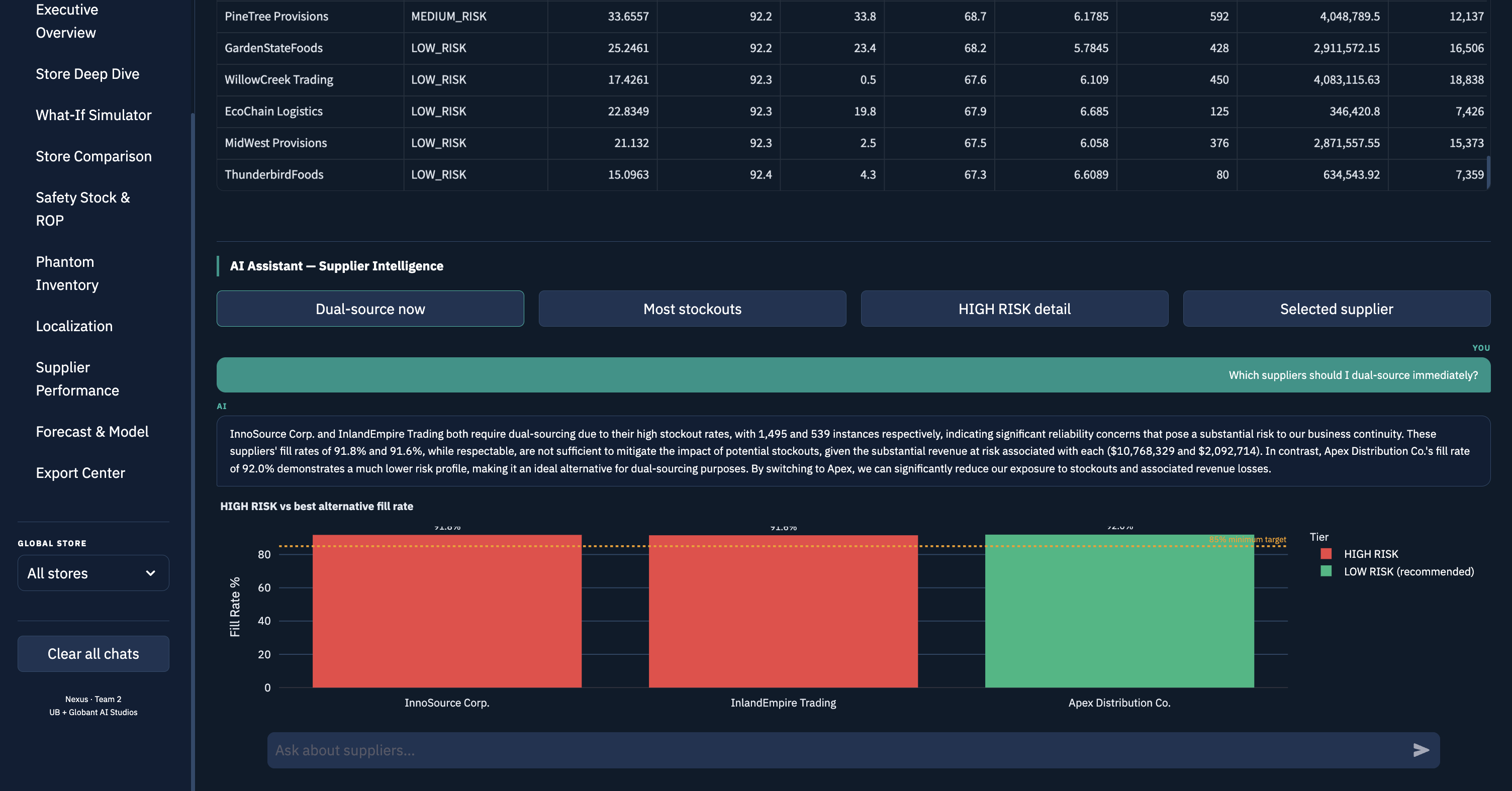
Supplier Performance
85-supplier dropdown. Fill rate vs reliability scatter with 85% threshold line. 4-factor scorecard bar chart. Risk tier assignment (HIGH/MEDIUM/LOW).
AI: "InnoSource Corp causing most stockouts — 1,495 events, $10.7M at risk. Fill 91.8%, late 56%, short 71.2%. Dual-source immediately. InlandEmpire also HIGH RISK."
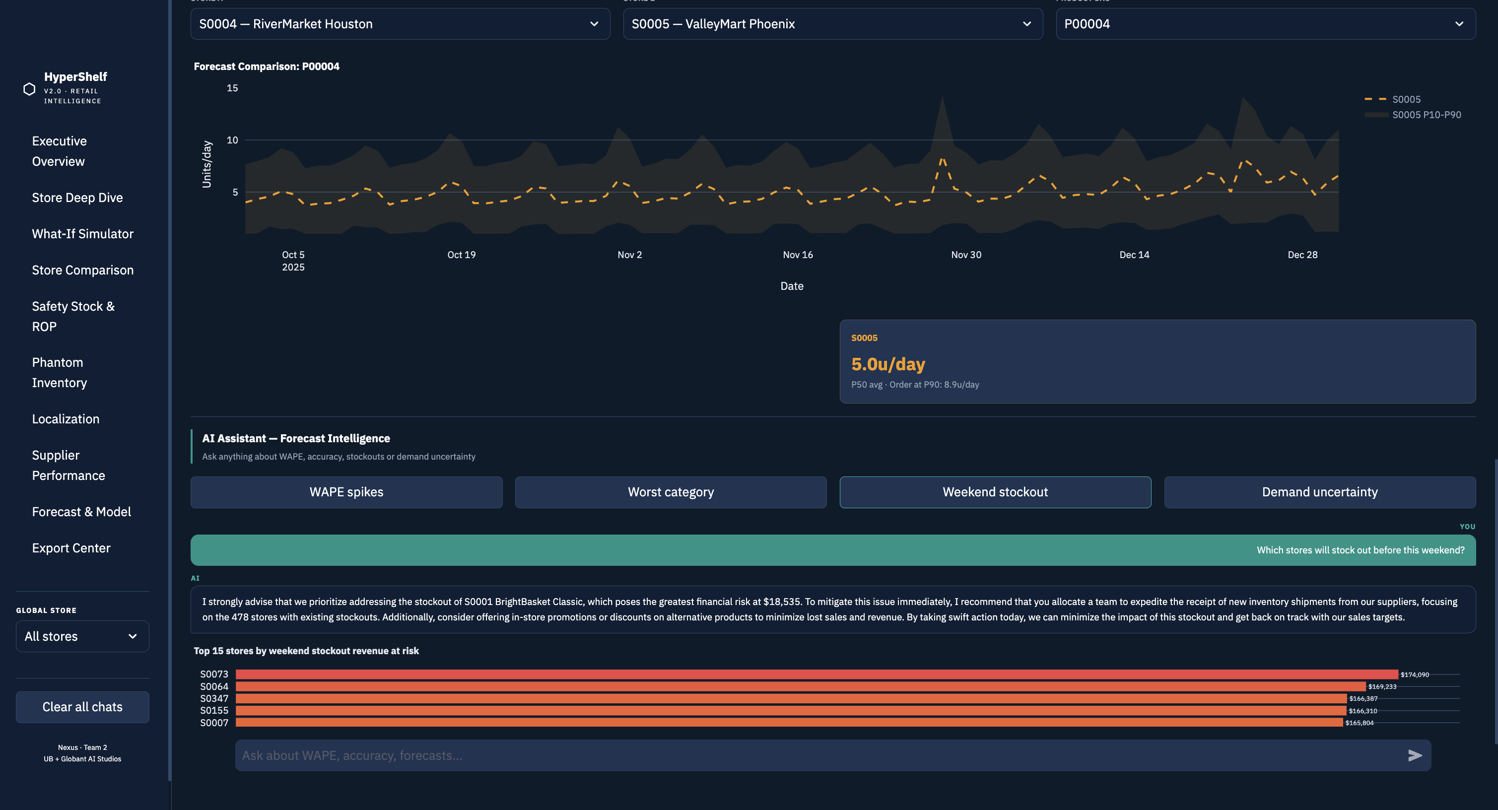
Forecast & Model
Forecast & Model
WAPE trend with spike detection. P10/P50/P90 demand band per SKU. Weekend stockout card. Category accuracy worst to best. Weekly bias monitoring.
AI: "Black Friday (Nov 24-30): WAPE 32.3%, Bias -1.72. Model over-predicted demand — stores cleared stock fast. For every 10 units sold, model predicted 17."
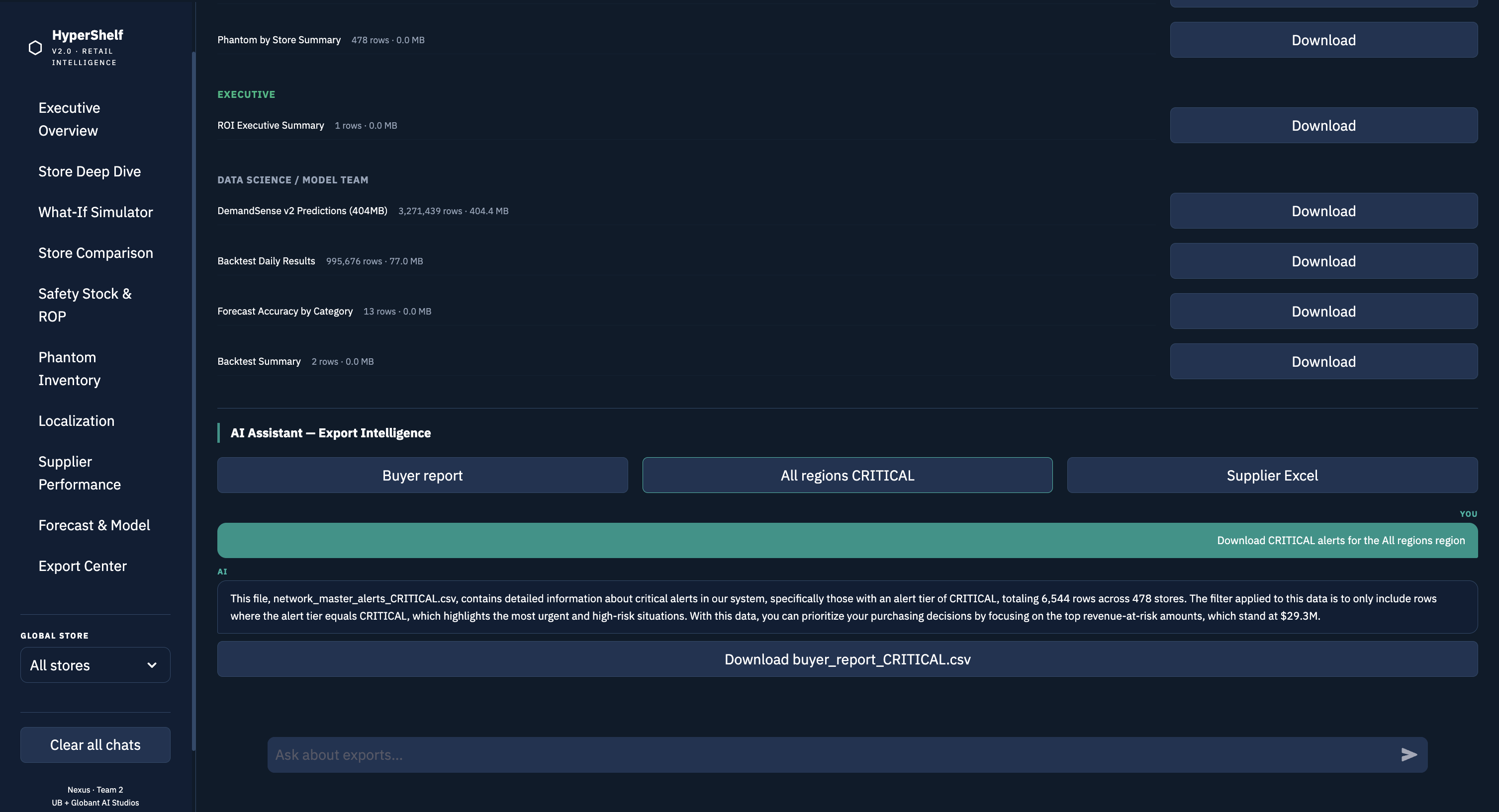
Export Center
Export Center
Role-based downloads (Store Manager / Buyer / Planner / Executive / Data Science). Excel supplier scorecard color-coded by risk tier. Region-filtered CRITICAL CSV.
AI: "Buyer report: 6,544 CRITICAL rows · 478 stores · $29.3M at risk. Sorted by revenue at risk desc. Download: buyer_report_CRITICAL.csv · Supplier Excel: red=HIGH RISK · 2 suppliers."
MLOps governance

Component-specific gates
not just LightGBM.

Production-grade AI systems gate every component, not just the headline model. Each part of the pipeline has its own evaluation criteria because each part fails in different ways: the forecasting model drifts, the phantom classifier silently drops recall, and the LLM starts routing to the wrong handler.

LightGBM (Forecast)
Champion/Challenger CI/CD
WAPE must improve vs V1. P90 must stay 88–92%. Zero regression in Beverages or Snacks (highest impact score categories).
Random Forest (Phantom)
Recall + F2 threshold
Recall is the primary gate — missing real phantoms (FN) costs money. F2 threshold from PR-curve. Precision is secondary.
LLM (LLaMA 3.2)
Routing accuracy tests
Unit tests verify WAPE questions hit forecast handler, replenishment questions hit replenishment handler. No hallucination on known store IDs or revenue figures.
Data Pipeline
Schema + freshness checks
Column presence validation on all CSVs. Freshness check on network_master_alerts.csv. Volume sanity check — if row count drops >10%, pipeline alert fires.
2 weeks
Scheduled retraining cadence. Challenger model trained on latest data, evaluated against champion before any promotion.
12 weeks
Rolling validation window for continuous training governance. Captures seasonal variation while remaining sensitive to recent drift.
WAPE worsens > 1.5 pts → emergency retrain
P90 exits 88–92% band → emergency retrain
Volume bias > 0.5u → emergency retrain
3 gates
Champion/Challenger promotion requires all three to pass: WAPE improved, P90 in band, zero category regression. All must pass simultaneously.
Outcomes

Numbers that move
in retail.

$275.6M
Revenue recovered vs old static reorder policy across all 478 stores
59.92% of total stockout losses recovered
188,143
Stockout events prevented vs MovingAvg30 baseline — Black Friday + Christmas backtest
8.33% reduction in stockout events
14.6%
WAPE improvement — 24.06% vs 28.19% baseline. LightGBM vs 30-day moving average on True Demand.
4.13 percentage points absolute improvement
+57 pts
P90 demand coverage improvement — 89.75% vs 32.7% legacy. The safety band now actually works.
Target 88–92% · achieved 89.75%
-0.148
Model bias — near zero means balanced forecasting. Slight under-prediction is safer than over-ordering in retail.
Target: within ±0.5 units
14,041
Phantom SKUs detected and queued for physical aisle verification across the network
High/Medium/Low confidence scoring
Tech stack

Built on open-source tools.
Designed for production.

LightGBM demand forecasting, Random Forest phantom detection, LLaMA 3.2 language interface, and a 10-page Streamlit dashboard — all running on a single machine with no cloud dependencies.

LGB
LightGBM
Gradient boosting demand forecasting. 22 features. 3.27M P10/P50/P90 predictions. WAPE 24.06%.
RF
scikit-learn RF
Random Forest phantom classifier. F2-optimised threshold. 14,041 candidates detected.
🦙
LLaMA 3.2 3B
Local inference via Ollama. Sub-2 second response. Zero API calls. Temperature 0.1/0.2.
ST
Streamlit
10-page dashboard on :8511. Standalone AI chat on :8501. Live ticker, gauges, chat bubbles.
Px
Plotly
All charts. Renders inside AI chat bubbles. Gauges, scatter, radar, bar, pie. Custom DL() theme.
Pd
Pandas + scipy
Every AI answer starts here. scipy.stats for Z-score, norm.cdf for service level calculations.
Run it yourself

Clone. Install.
Run.

Setup

git clone https://github.com/Nirwade/HyperShelf_Retail-AI-project
cd HyperShelf_Retail-AI-project
conda create -n retail-ai python=3.10
conda activate retail-ai
pip install -r requirements.txt
python scripts/setup_sample_data.py
ollama pull llama3.2:3b && ollama serve

Launch

# Dashboard — 10 pages with AI
python -m streamlit run streamlit_app/app.py --server.port 8511
# Standalone AI chat
python -m streamlit run streamlit_app/llm_chat.py --server.port 8501
Dashboard
localhost:8511
10 pages · AI per page · live alerts
AI Chat
localhost:8501
8 tools · conversational · morning briefing

Want to see it live?

Request a demo session to walk through all 10 pages and both AI interfaces. Or download the full project book for the complete methodology.

Request a demo → Project Book ↓
Project information

Version 1 & 2 — All Access Links

Version 1 — Original Team Dashboard
DASHBOARD URL
http://localhost:8050
Requires app_dashboard.py to be running
CODE REPOSITORY
GitHub — HyperShelf
Private repository — team access required
DOCUMENT VERSION
Version 1.0 Final — April 2026
Version 2 — DemandSense v2
PORTFOLIO WEBSITE
nirwade.github.io
Live — interactive showcase with demos
DASHBOARD URL
http://localhost:8511
10-page AI dashboard — requires Streamlit and data files
CODE REPOSITORY
github.com/Nirwade/HyperShelf_Retail-AI-project
Public — full source code with README and sample data
DOCUMENT VERSION
Version 2.0 Final — May 2026
Nexus Team 2 · University at Buffalo · Globant AI Studios
HyperShelf DemandSense v2 · UB + Globant AI Studios · Nexus Team 2 · Built May 2026